Lotka–Volterra Case Study#
Data source:#
This example only uses simulated dataset to show the efficacy of InvODE.
[1]:
import numpy as np
from scipy.integrate import odeint
import matplotlib.pyplot as plt
import os
import sys
import scipy.io
[2]:
# Get path to MCMCwithODEs_primer (3 levels up)
project_root = os.path.abspath(os.path.join(os.getcwd(), '..','..','..'))
sys.path.insert(0, project_root)
In this example, we simulate the classic Lotka-Volterra model using chosen values of parameter set, add additive Gaussian noise to the time series and treat this in-silico time series as raw data for pointwise inference. The model of prey, \(x\) and predator \(y\) is given by,
\[\frac{dx}{dt} = \alpha x -\beta xy\]
\[\frac{dy}{dt} = \delta xy -\gamma y\]
[3]:
def lotka_volterra(z, t, params):
    x, y = z
    alpha = params['alpha']
    beta = params['beta']
    delta = params['delta']
    gamma = params['gamma']

    dxdt = alpha * x - beta * x * y
    dydt = delta * x * y - gamma * y
    return [dxdt, dydt]
[4]:
true_params = {
    'alpha': 1.0,    # prey growth rate
    'beta': 0.1,     # predation rate
    'delta': 0.075,  # predator growth per prey eaten
    'gamma': 1.5     # predator death rate
}

t = np.linspace(0, 20, 200)
z0 = [40, 9]  # initial population: 40 prey, 9 predators
[5]:
true_sol = odeint(lotka_volterra, z0, t, args=(true_params,))
noisy_data = true_sol + np.random.normal(0, 1.0, true_sol.shape)
Fitting the dataset with InvODE#
[6]:
def simulate_model(params):
    sol = odeint(lotka_volterra, z0, t, args=(params,))
    return sol  # shape: (N, 2)

def mse(output):
    return np.mean((output - noisy_data)**2)
In this example, we show that only a wide parameter bound is sufficient to infer parameters. Unlike many other packages, we do not need to provide an initial guess. The paramter range is kept wide intentionally for demonstration.
[7]:
param_bounds = {
    'alpha': (0.5, 10),
    'beta': (0.05, 0.9),
    'delta': (0.05, 0.9),
    'gamma': (1.0, 5.0)
}
[8]:
import sys
sys.path.append('./..')  # or absolute path if needed

from invode import ODEOptimizer, lhs_sample
[9]:
# Run optimizer
optimizer = ODEOptimizer(
    ode_func=simulate_model,
    error_func=mse,
    param_bounds=param_bounds,
    seed=42,
    num_top_candidates=3
)
[10]:
optimizer.fit()
Fitting Progress: 100%|█████████████████████████████████████████████████| 10/10 [00:03<00:00, 3.08it/s]
Refining params: {'alpha': 0.5483310416214465, 'beta': 0.068028770810073, 'delta': 0.1451018918331013, 'gamma': 3.1481636450536428}
Refining params: {'alpha': 0.8216385700908369, 'beta': 0.12479204383819222, 'delta': 0.0616377161233344, 'gamma': 1.615577581450748}
Refining params: {'alpha': 1.088028953494527, 'beta': 0.24201471359553078, 'delta': 0.10339353925892915, 'gamma': 1.6535395505316968}
[10]:
({'alpha': 0.9998973552849139,
  'beta': 0.09995621865139477,
  'delta': 0.07482275016126995,
  'gamma': 1.4972199684549248},
 0.9454500024300705)
[11]:
optimizer.summary()
🔍 ODEOptimizer Summary:
  ode_func: simulate_model
  error_func: mse
  param_bounds: {'alpha': (0.5, 10), 'beta': (0.05, 0.9), 'delta': (0.05, 0.9), 'gamma': (1.0, 5.0)}
  initial_guess: {'alpha': 5.25, 'beta': 0.47500000000000003, 'delta': 0.47500000000000003, 'gamma': 3.0}
  n_samples: 100
  num_iter: 10
  num_top_candidates: 3
  do_local_opt: True
  local_method: L-BFGS-B
  shrink_rate: 0.5
  parallel: False
  local_parallel: False
  verbose: False
  verbose_plot: False
  seed: 42
  best_error: 0.9454500024300705
  best_params: {'alpha': 0.9998973552849139, 'beta': 0.09995621865139477, 'delta': 0.07482275016126995, 'gamma': 1.4972199684549248}
[12]:
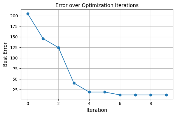
optimizer.plot_error_history()
[13]:
optimizer.best_params
[13]:
{'alpha': 0.9998973552849139,
 'beta': 0.09995621865139477,
 'delta': 0.07482275016126995,
 'gamma': 1.4972199684549248}
[14]:
optimizer.best_error
[14]:
0.9454500024300705
[15]:
history = optimizer.get_top_candidates_history()

# Example: print best candidate from each iteration
for i, candidates in enumerate(history):
    print(f"Iteration {i+1}: Best error = {candidates[0][1]:.4f}")
Iteration 1: Best error = 204.6680
Iteration 2: Best error = 145.7022
Iteration 3: Best error = 124.5489
Iteration 4: Best error = 40.5091
Iteration 5: Best error = 19.2365
Iteration 6: Best error = 51.9826
Iteration 7: Best error = 12.4050
Iteration 8: Best error = 32.4487
Iteration 9: Best error = 50.0270
Iteration 10: Best error = 26.6829
If we wanted to explore what parameters were sampled and chosen on the way towards optimization, we can dig into it.
[16]:
df = optimizer.get_top_candidates_table()
print(df)
    iteration  rank       error     alpha      beta     delta     gamma
0           1     1  204.667960  4.635283  0.548670  0.272194  3.750834
1           1     2  218.967236  3.948483  0.639474  0.266935  3.296262
2           1     3  224.830375  3.143117  0.334123  0.277048  2.619616
3           2     1  145.702157  6.541759  0.669410  0.176117  3.965542
4           2     2  150.452967  3.694805  0.448981  0.095968  2.381629
5           2     3  151.425265  4.592497  0.524295  0.146545  3.973435
6           3     1  124.548898  1.667789  0.482981  0.145486  1.406716
7           3     2  126.479216  3.239774  0.298372  0.075456  1.800184
8           3     3  139.599956  4.021883  0.458061  0.139802  3.099533
9           4     1   40.509116  1.501547  0.157396  0.096360  1.188872
10          4     2   67.987344  1.113214  0.313581  0.092433  1.601306
11          4     3  108.088022  1.100925  0.343522  0.162367  2.142834
12          5     1   19.236542  1.221271  0.188816  0.071793  1.239034
13          5     2   64.401317  0.757612  0.173760  0.208879  2.972718
14          5     3   77.198631  1.050500  0.111615  0.069860  1.256183
15          6     1   51.982562  1.509966  0.133063  0.101699  1.197996
16          6     2   54.708467  1.240501  0.234195  0.096619  1.421084
17          6     3   64.200622  1.195991  0.279601  0.052210  1.229068
18          7     1   12.404973  0.818549  0.082426  0.081083  1.861002
19          7     2   18.786631  0.732057  0.097124  0.129818  2.363097
20          7     3   26.713208  1.454759  0.170437  0.073618  1.060169
21          8     1   32.448662  1.102807  0.121274  0.113574  1.619607
22          8     2   33.477406  1.566777  0.165080  0.082514  1.096553
23          8     3   46.206608  0.760460  0.185158  0.108213  2.202863
24          9     1   50.027043  0.680582  0.058895  0.122742  2.325857
25          9     2   81.652486  1.078495  0.083594  0.135380  1.802685
26          9     3   89.614766  0.916940  0.247304  0.187210  2.566774
27         10     1   26.682906  0.548331  0.068029  0.145102  3.148164
28         10     2   36.568860  0.821639  0.124792  0.061638  1.615578
29         10     3   63.653644  1.088029  0.242015  0.103394  1.653540
[17]:
best_params = optimizer.best_params
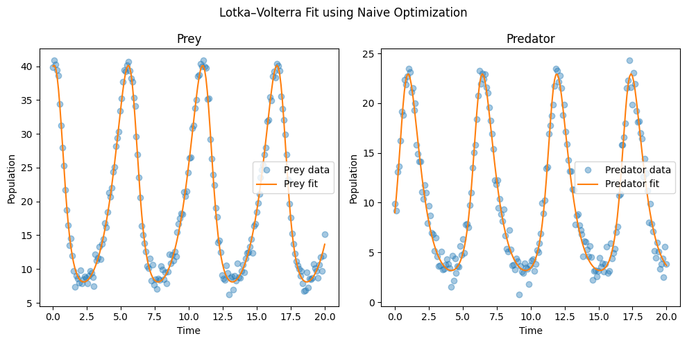
[18]:
best_fit = simulate_model(best_params)


plt.figure(figsize=(10, 5))
plt.subplot(1, 2, 1)
plt.plot(t, noisy_data[:, 0], 'o', alpha=0.4, label='Prey data')
plt.plot(t, best_fit[:, 0], label='Prey fit')
plt.xlabel("Time")
plt.ylabel("Population")
plt.legend()
plt.title("Prey")

plt.subplot(1, 2, 2)
plt.plot(t, noisy_data[:, 1], 'o', alpha=0.4, label='Predator data')
plt.plot(t, best_fit[:, 1], label='Predator fit')
plt.xlabel("Time")
plt.ylabel("Population")
plt.legend()
plt.title("Predator")

plt.suptitle("Lotka–Volterra Fit using Naive Optimization")
plt.tight_layout()
plt.show()
[19]:
from invode import ODESensitivity
[31]:
sensitivity = ODESensitivity(ode_func=simulate_model,error_func=mse)
[32]:
sensitivities = sensitivity.analyze_parameter_sensitivity(df)
[33]:
# Identify most consistently sensitive parameters
summary['mean_abs_sensitivity'] = summary.abs().mean(axis=1)
print(summary.sort_values('mean_abs_sensitivity', ascending=False))
       correlation  rank_correlation  variance  mutual_info  \
beta      1.000000          1.000000  0.837219     1.000000
alpha     0.939654          0.821020  0.705869     0.890829
delta     0.882231          0.691107  1.000000     0.528090
gamma     0.739286          0.660998  0.000000     0.000000

       mean_abs_sensitivity
beta               0.959305
alpha              0.839343
delta              0.775357
gamma              0.350071
[ ]: